Снижение размерности: метод t-SNE

import numpy as np
import matplotlib.pyplot as plt

# Смоделируем плоскость
def f(x,y):
  return (x - 1.0)**2 + (y+1)**4

x = np.linspace(-3.4, 3.4, 500)
y = np.linspace(-1.5, 1.5, 500)
X,Y = np.meshgrid(x,y)
Z = f(X,Y)

# Создание датасета точек на плоскости
xmin, xmax = -3.4, 3.4
x1 = np.linspace(xmin, xmax, 500)
fx = np.sin(x1)
dots = np.vstack([x1, fx]).T
noise = 0.2 * np.random.randn(*dots.shape)
dots += noise

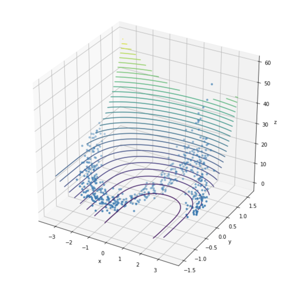
# Добавим третье измерение
def zfun(xy):
    x, y = xy[0], xy[1]
    z = (x - 1.0)**2 + (y+1)**4
    noise = 0.2 * np.random.randn(*z.shape)
    z += noise
    return z
z = zfun(dots.T)
dots_3d = np.hstack([dots, z.reshape((len(z),1))])
XYZmat = dots_3d.T

fig = plt.figure(figsize=(10, 10))
ax = plt.axes(projection='3d')
ax.contour3D(X, Y, Z, 30, )
ax.scatter(XYZmat[0], XYZmat[1], XYZmat[2], s = 10, marker='o')
ax.set_xlabel('x')
ax.set_ylabel('y')
ax.set_zlabel('z')
fig.show()

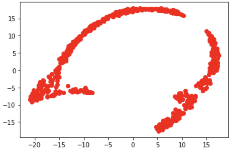
from sklearn.manifold import TSNE

# Используем метод t-SNE
tsne = TSNE(n_components=2, perplexity=40)
# perplexity – указываем сколько точек нам учитывать в окружении для подсчета 
# вероятностных расределений
tsne.fit(dots_3d)
newZ = tsne.embedding_

plt.scatter(newZ[:, 0], newZ[:, 1], c='r')